Introduction

In my previous post, I described a technique for explainability that involves decomposing the intermediate hidden states of a language model into a set of source and target states. By doing so, we can retrieve the exact contribution of each token to the hidden state of another token, which can then be used to explain the output from any number of downstream tasks. While writing it, I thought about how this can be applied to transformer models that accept inputs of various types (images, audio, etc.). While this does bring various unique challenges, I was finally able to write an implementation of multimodal decomposition that creates cross-modality explanations.

Why is this important?

Multimodal language models are becoming ubiquitous and all current methods for transformer model explainability are unimodal, with image explanations being considered independently of text explanations. In the paper “Rethinking Explainability in the Era of Multimodal AI”, Chirag Agarwal argues that “unimodal explanations systematically misrepresent and fail to capture the cross-modal influence that drives multimodal model decisions, and the community should stop relying on them for interpreting multimodal models.” 1. Becuase of this, there is a strong need to develop model techniques that can create unified explanations for both text and other model inputs.

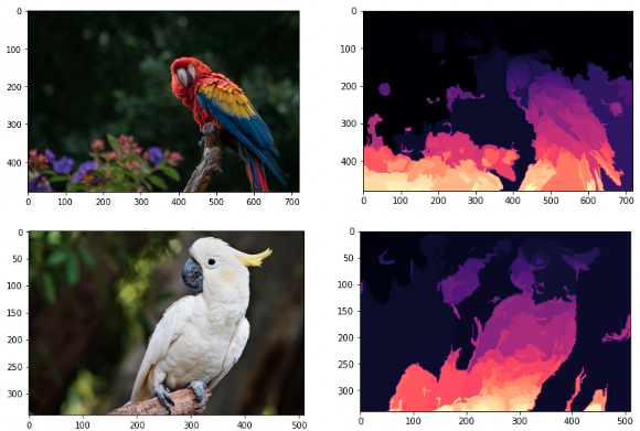
Caption: A set of 2 images with explanation heatmaps using the XRAI technique 3. Sections containing a bird are highlighted in red while non-bird sections are black.

Multimodal Decomposition Basics

As described previously, decomposition works due to the fact that most operations performed by a transformer model are linear. This means that we can run each model step on the decomposed hidden state while still retaining the ability to collapse it into the undecomposed version. By handling the nonlinear MLP step using linear approximation, we are able to run through the entire model and get a decomposed, fully attributed hidden state from the model.

Since the vision encoders used by multimodal language models are also transformer-based, the same logic can be used to create a decomposed image embedding. After the image embedding is retrieved, a linear transformation is applied to the image embedding to obtain a set of tokens with the embedded image.

Difficulties

While the overall logic behind multimodal decomposition is basic, the actual implementation of it has a few complications:

Space Complexity

One obvious difference between a piece of text and an image is that an image is two-dimensional. What this means for decomposition is that a decomposed representation of an image is much larger than any decomposed text embedding. For example, a 64 x 64 grid of image patches is decomposed into 64 x 64 x 64 x 64, or 16,777,216 pairwise attributions. If we use a model with a hidden size of 768 and a dtype of float32, the decomposed tensor would use approximately 51GB of RAM and take an absurdly long time to calculate. For large text inputs, this problem can be mitigated by decomposing a subset of the tokens, since many tasks use only the final token’s hidden state. However, this is not possible for images, since we pretty much always want to decompose the entire image.

To solve this, I added a ‘scaling factor’ to the decomposed embedding that pools square sets of image patches before decomposing. In our 64 x 64 example, a scaling factor of 2 would use a 2x2 pooled grid of image patches, making the decomposed embedding have a size of 64 x 64 x 32 x 32. This reduces the size of the tensor by a factor of 4, meaning it only takes up 12GB of space. This scaling factor can be dynamically adjusted depending on available memory.

Integration With Text Embeddings

Because we rescale the size of the images, sizes of the source and target dimensions no longer match directly. For example, if we have 10 text tokens and 64 image tokens with a scaling factor of 2, the full decomposed embedding would be of size (10+64) x (10+32) = 74 x 42. Additionally, this relationship between source and target tokens can be either one-to-many OR many-to-one, since our scaling factor works independently of the image scaling that occurs during regular model inference (i.e. if the regular model scaling reduces to 8 image tokens and our scaling factor reduces to 16).

Results

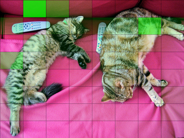
I modified the SmolVLM-256M-Instruct model for decomposition in order to test performance. Since I’m running the model on a laptop with limited memory, I set the scaling factor to 4 to get an 8x8 grid of image attributions along with the full set of text attributions. I used the following image along with the text “Describe this image.” as input and retrieved a (truncated) response.

Caption: The sample input used for multimodal decomposition. It contains two cats lying down on a pink blanket.

User: Describe this image.

Assistant: The image depicts two cats lying on a pink blanket. The cat on the left is smaller and has a lighter color, while the cat on the right is larger and has a darker color. Both cats are lying on their sides, facing opposite directions. The smaller cat is positioned on the left side of the image, while the larger cat is positioned on the right side.\n\nThe background of the image is a pink blanket, which is likely a blanket used for pets. The blanket has a soft

I then ran the entire text through the decomposed model and calculated the delta log-probability for each token as an explanation metric. Specifically, I looked at the token importances to generate the token following “depicts”.

Caption: Text explanation for the above sequence of text. Various image tokens are highlighted with different shades of red, with the darkest tokens being the phrase “The image depicts”.

By transforming the image tokens back into image patches, we can visualize the importance of each section of the image:

Caption: Explanations for each section of the above image. A few sections are highlighted in green, with most sections being completely transparent.

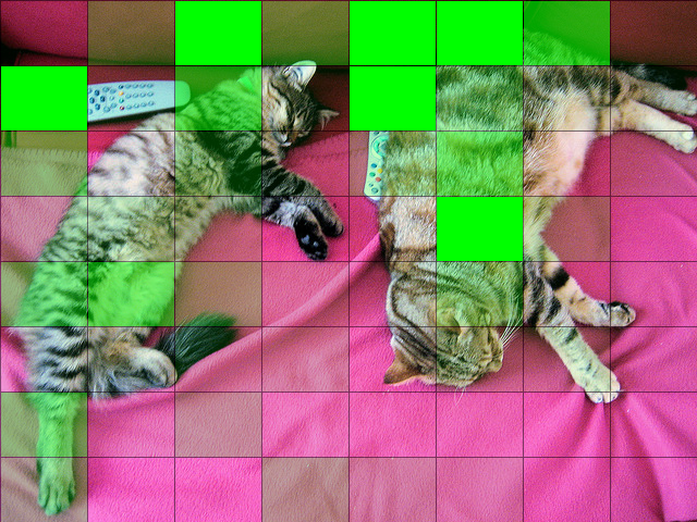
Interestingly, we can see that very few patches of the image were important for generating the word “two”. In fact, we observe the same pattern for every generated token. In order to get a more complete picture, we can try looking at the average attribution across multiple tokens. If we look at the maximum image attributions for the model to generate the word “cat” or “cats”, we can observe whether the model utilizes the image sections that contain a cat:

Caption: Explanations for each section of the above image. More sections are highlighted in green, most of which are sections containing a cat.

From the image, we can see that most of the time the model does use sections containing a cat to generate the word ‘cat(s)’. However, it’s not as clear as other image-only or text-only explainability metrics like XRAI. I also noticed that the earlier image tokens tend to have higher relevance than later ones, potentially showing how a model might use exclusively the first section that matches, rather than utilizing all relevant image sections. This could also interfere with the delta log-probability metric we’re using. An individual section containing a cat might be marked as low relevance because ablating that single section causes the model to use all of the other ‘cat’ sections. This provides an explanation for the apparent noisiness of each explanation.

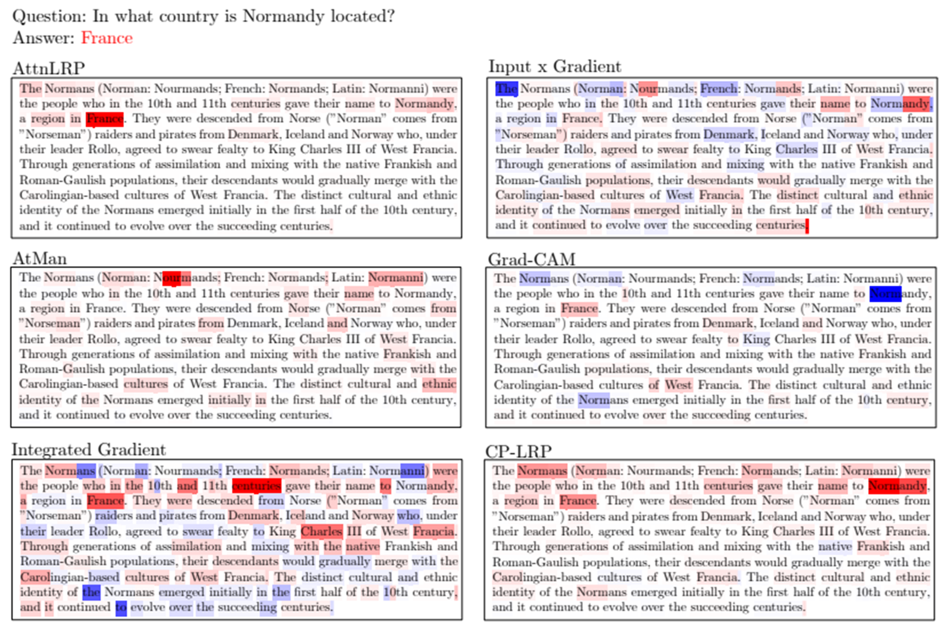
Caption: A set of model explanations for the same question using various techniques 2.

Conclusion

Decomposition gives us the ability to create explanations for the outputs of multimodal transformer models, which is crucial for understanding the behavior of said models. As far as I know, this is the first technique that directly computes attributions between image and text data. These explanations tend to be fairly noisy when it comes to images, highlighting the need for more robust multimodal explainability techniques.

In the future, I hope to continue to explore decomposition in both text and image scenarios. To understand the quality decomposition compared to other techniques, I plan on using the OpenXAI library and leaderboard. I also hope to apply this technique to larger models, as the quality of the explanation could scale with the quality of the model response itself.

References

Machine Learning Interpretability

I won’t spend much time going over the importance of interpretability in machine learning, but a couple recommended resources for learning about it are Cristoph Molnar’s textbook “Interpretable Machine Learning” and Chapter 4 of the University of Helsinki’s MOOC on Ethical AI ^{1 2}. Broadly, interpretable models allow us to provide accountability for affected individuals, be transparent about the reasons behind a model’s prediction, and improve the model’s performance.

Language Model Interpretability

Several methods exist that attempt to create human-interpretable explanations for a model’s output, including gradient-based, vector-based, and other methods [6]. However, the one that I’ll be focusing on in this blog is called “Token-Wise Decomposition” from Oh & Schuler ³.

Caption: A set of model explanations for the same question using various techniques ⁴.

Background

Autoregressive language models all perform a specific set of operations on a number of input tokens in order to make a prediction. The result of these operations is a kind of embedding of the input text, called a hidden state. These operations are repeated over a set number of layers to retrieve the final hidden state of the model.

1. Text Embedding: The model creates an initial hidden state by embedding each token individually.
2. Normalization: Each token’s hidden state vector is normalized according to a specific model. For example, LLaMA uses Root Mean Squared normalization.
3. Self-Attention: An ‘attention matrix’ is created from the hidden state of each token, which adjusts each token depending on the others present in the sequence [^*].
4. MLP: A two-layer neural network is applied to each token’s hidden state, typically including ‘upscaling’, ‘downscaling’ and nonlinear activation function.

Once these steps are performed for each layer, the final hidden state is then passed to a module specific to a given task. These modules, or ‘heads’, can be used for virtually any machine learning task, such as token or sequence classification, information retrieval, or token generation.

Decomposition Steps

The idea behind decomposition is that each token’s hidden state can be broken down, or ‘decomposed’, into a 2-dimensional diagonal matrix containing that same hidden state. Then, by performing each of the steps defined above, we can retrieve the exact value of each token’s contributions to every other token’s hidden state. As we progress through the model, we can retrieve the original hidden state for each target token by simply summing over the second (source) dimension.

For example, if we have a sequence of 10 tokens with a hidden state size of 796, our usual input would be a tensor of shape (10, 796). When we decompose the same hidden state, we would instead have a tensor of shape (10, 10, 796) with each of the 10 values mapped to the 10 x 10 diagonal with 0 everywhere else. Additionally, we create a ‘bias’ tensor of 0s with shape (10, 796) that tracks the hidden state transformations that cannot be attributed to an individual token.

Caption: Schematic showing how traditional models calculate a single hidden state vector for each token while a decomposed model creates a pairwise set of hidden states that sums to the undecomposed representation ³.

Once we create the initial decomposed hidden state, we can move through steps 3 and 4 of the model normally by taking advantage of an interesting property of linear functions. When a linear function like matrix multiplication is applied to both a decomposed hidden state matrix A and the undecomposed version B, the resulting matrix AC remains a decomposed version of AB. Since normalization and self-attention both apply linear functions to each matrix, we can run through each of those steps without modification.

Step 4, however, poses a problem. This is because the activation function of the MLP layer is usually nonlinear, meaning the decomposition is broken when passing through it normally. Oh and Schuler solve this by taking a local linear approximation of this activation function at each location, which preserves this relationship if the activation function is differentiable almost everywhere ³.

Since each of our steps now can be applied to the decomposed version, we’re able to run through the entire model to retrieve the decomposed hidden states at each layer. From there, we can apply any linear head to these hidden states to create a model output that preserves each token’s relationship with each other.

Text Generation Outputs

To explain the generation of a single token, Oh and Schuler define a specific importance measure, called ∆LP. Since the output of a language model is a probability distribution over all possible tokens to generate, it follows that a token is important if removing that token’s contribution has a significant effect on the probability of generating the next token. This is defined formally using the following equation:

where \(w_i\) is the token at index i.

Classification Outputs

Explaining the output from a classification head is very simple, since it’s usually just a linear function of the pooled hidden states of the model. Pooling involves combining the hidden states for each token into a single state that represents the sequence as a whole. Because these functions are also linear, we can apply the classification weights to the decomposed and unpooled hidden states to retrieve a logit value for each source and target token. Then, we can define each source token’s contribution to the final prediction as the sum of all ‘target’ tokens plus the bias term multiplied by the model’s pooling weight. For example, if our pooling method takes a simple mean across all tokens, the contribution of source token j is defined as:

\(Contribution_j =\sum^{E}_{e=1}\frac{\beta_et_{e,l}}{L-(l-1)}\),

with \(E\) being the hidden state dimension of the model, \(\beta_e\) being the classifier’s weight at dimension \(e\), \(L\) being the sequence length, and \(t_{e,l}\) being the target hidden state of token \(l\) at dimension \(e\).

Example: Groundedness Detection (NLI)

To show how decomposition works, I used an example from the ‘AggreFact’ dataset, containing a set of documents and claims with the goal of predicting whether a claim is supported by the given document [9]. I chose this task specifically since it is much more difficult than other tasks for generative models like content safety classification or jailbreak detection. Using Qwen 3 0.6B with the same prompt as MiniCheck 7B, I retrieved the token importance for generating the token ‘No’.

Caption: Image showing a sample prediction, with token importance being represented by the highlighted color.

From this visualization, we can see that the instructions in the system prompt had the most effect on the model’s response. In addition, the token for ‘more’ in the phrase ‘more than 21 km’ as well as ‘19’ in ‘19 km north’ were significant. Because of this, we conclude that the model is using the correct tokens in the input to generate it’s response.

However, this also highlights a flaw in using generative models for classification tasks. Despite the model using the correct tokens for its response, we can see that the majority of significant tokens are from the instructions in the prompt, as well as the special tokens related to the ‘chat’ template the model follows. If we can train a classification model to directly identify ungrounded claims rather than relying on generated tokens, we could likely improve its performance as well as interpretability.

Optimizing Decomposition Performance

Since we’re decomposing a set of N tokens into N^2 pairs of tokens, the performance of the transformer model suffers from quadratic time complexity with respect to the number of tokens. When comparing it to a another technique (LXR), we see that decomposition performs better on a smaller number of tokens, but eventually performing worse at around 360 tokens of input since LXR computes explanations in linear time. With this basic implementation, decomposition doesn’t scale well enough to be used in any practical application.

Caption: Runtime comparison of LXR and decomposition. LXR shows a linear trend based on the number of tokens while decomposition shows a quadratic trend.

A large reason for this difference is that decomposition computes the token attribution for all pairs of tokens, while LXR works only on a single token at a time. If we were able to reduce the number of tokens being decomposed, decomposition could become more viable. In addition to this, we can decide to skip a certain number of layers inside the model to speed up computation. This has the effect of increasing the magnitude of the bias term when compared to the decomposed version, meaning we are able to attribute less of the overall hidden state to each individual token. However, we find that the relative attribution between tokens for each hidden state remains the same when compared to the full model. Because of this, the token decompositionwhen skipping layers remains relevant to the overall interpretability of the model.

Caption: Plot showing the runtime of a decomposed model when compared to the baseline model when skipping a certain proportion of layers and analyzing a certain proportion of tokens.

After modifying the decomposition code to allow for any number of tokens to be analyzed and to skip any number of layers, we compare the overall performance to our baseline for Qwen 3 0.6B. From the above plot, we see that performance similar to our baseline can be achieved by aggressively reducing the number of tokens analyzed and by skipping most layers in the model.

Conclusion

Compared to other explainability methods for language models, decomposition is significantly more flexible and allows us to see exact contributions to each hidden state. Because of this, I think that it’s a super promising method for understanding the outputs of any transformer-based language model.

This method could also work for vision-based transformers or multimodal models, but the two-dimensional nature of images exacerbates the memory and computation problems described earlier. Since we can’t reduce the decomposed pixels in an image in the same way as with text, other workarounds must be developed instead.

References